In Chapter 9, I mentioned that a job of physicists doing quantum mechanics is finding the definite-energy eigenfunctions for problems with various potential energy distributions. We saw the definite-energy eigenfunctions for the potential energy distribution representing a one-dimensional box. In this chapter, we will see a few of the definite-energy eigenfunctions for an electron in a three-dimensional hydrogen atom.

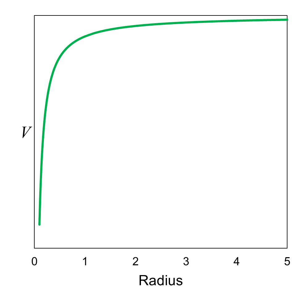
Figure 21 shows the potential energy distribution for the problem. This is the same distribution we saw in Chapter 8 where we learned about the relationship between force and potential energy. The difference in the figure is that we are using radius instead of x for position. The centrally located proton in the nucleus of the hydrogen atom is at radius = 0. The figure shows the electron’s potential energy as a function of distance (radius) from the proton.

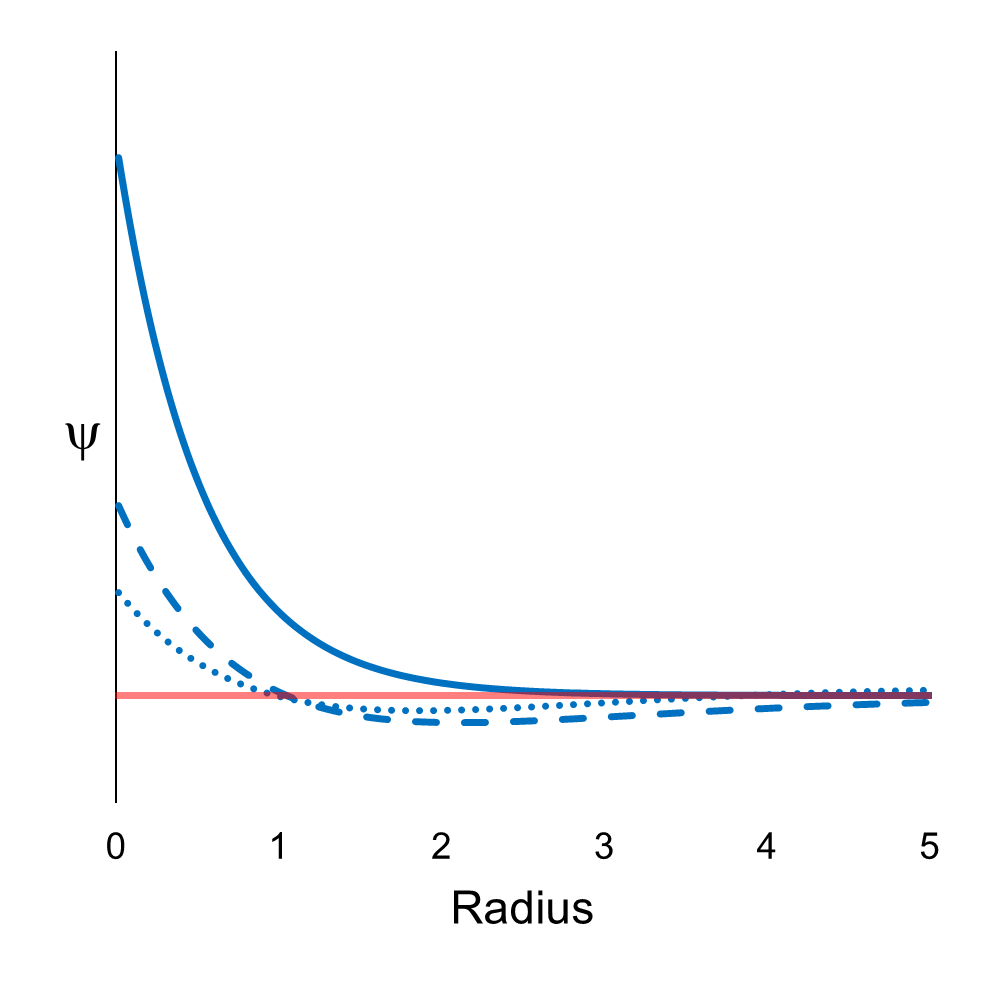
Figure 22 shows the eigenfunctions ψ corresponding to the first three definite energies: E₁ (solid line), E₂ (dashed line), and E₃ (dotted line). The imaginary part (red line) is zero for all three. (Note that these eigenfunctions are for electrons with zero angular momentum. Electrons can also be in configurations with nonzero angular momentum. Also, note that for each radial position, there is a corresponding spherical surface available for the electron. This needs to be accounted for when evaluating the probability of finding the electron, upon measurement, at any radial position.)

The electron in a hydrogen atom is confined, though not 100% confined like an electron in a box. The electron in a hydrogen atom is only partially confined by the electrostatic attraction between it and the proton. Still, the partial confinement is enough to result in the quantization of the possible values of definite energy. In other words, the possible values of definite energy are discrete, not continuous.

As you may have guessed, the wavefunction Ψ for an electron in a hydrogen atom can be expressed as a superposition of the definite-energy eigenfunctions, i.e., as a summation of definite-energy eigenfunctions ψ multiplied by probability amplitudes c.

Ψ = ∑c_Eψ_E     over all the possible definite energies E

We end with an example of how quantum mechanics explains how something works. Spectroscopy is a way to identify matter based on the wavelengths of the electromagnetic radiation the matter absorbs or emits. We will focus here on the emission part. Our understanding of how spectroscopy works relies on our understanding of the quantization—due to confinement—of the possible values of definite energy for electrons in atoms.

If a hydrogen atom is left alone for long enough, the electron will find itself in the ground state represented by a wavefunction equal to the eigenfunction corresponding to definite energy E₁. Suppose we heat-up a bunch of hydrogen atoms, putting their electrons’ wavefunctions into superpositions including higher-energy eigenfunctions. The excited electrons will eventually give up energy and fall back into lower-energy eigenstates. When an electron falls from a higher to a lower energy eigenstate, it emits a photon. The energy of the photon is equal to the difference between the two electron energy eigenstates.

For example, suppose an electron falls from the eigenstate with energy E₃ to the eigenstate with energy E₂. The energy difference E₃ − E₂ = 3 × 10⁻¹⁹ Joules. A photon with this energy has a wavelength of 6563 Angstroms, which we see as a red color. Electrons falling from and to different energy eigenstates emit photons with different wavelengths. Figure 23 shows the visible (with the naked eye) emission spectrum of hydrogen. Notice the red spectral line on the right. This is the one with a wavelength of 6563 Angstroms. There are other spectral lines with shorter and longer wavelengths that are outside the visible range.

Other kinds of atoms have different definite-energy eigenstates and therefore different emission spectra. One way to tell what elements are in something is to heat it up and observe the wavelengths of the spectral lines.