Let’s put an electron inside a box. Though a box has three dimensions—length, width, and height—we will only consider one dimension, the length, which we will align with the x-axis. The length of the box is one Angstrom, which is roughly the size of a hydrogen atom.

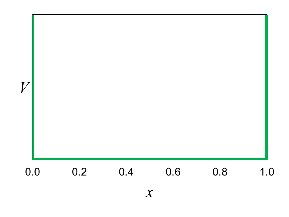
Figure 17 shows the potential energy distribution representing the box. Inside the box, the potential energy is zero. At both walls of the box, x = 0 and x = 1, the potential energy rises abruptly toward infinity. We learned in the previous chapter that force is equal to how much the potential energy changes over a small increment of distance. At the walls of the box, the force is extremely large. The potential energy goes from zero to infinity over an infinitesimal distance. The force at the walls is so great that the electron cannot escape from the box.

A special thing happens when quantum entities are confined like this. The possible, measurable values of definite energy E become discrete (or quantized) instead of continuous. This is different from what we saw before for position and momentum. The possible values of definite position and definite momentum are both always continuous (even though we treated them as discrete in Chapters 4 and 5 for convenience).

The discrete definite-energy values for confined quantum entities have corresponding definite-energy eigenfunctions ψ. One job of physicists doing quantum mechanics is to find the definite-energy eigenfunctions for problems with various potential energy distributions.

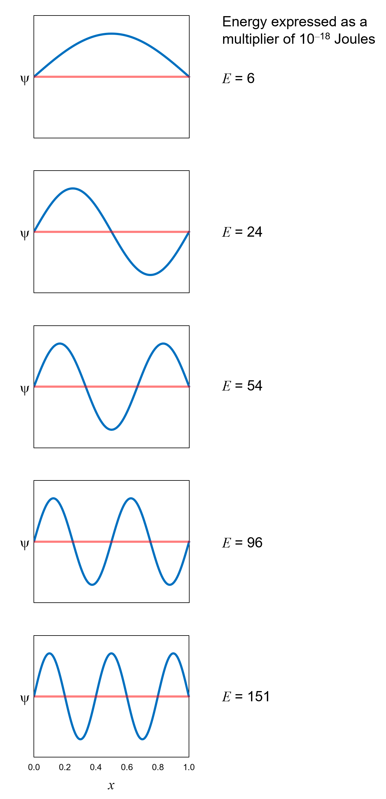
The definite-energy eigenfunctions for an electron in a box have been found. Figure 18 shows the eigenfunctions corresponding to the first five definite energies. Notice four things:

• The definite-energy eigenfunctions are all zero at the walls of the box. The electron cannot be right at a wall because of the enormous repulsive force at each wall. Because the electron cannot be at each wall, the eigenfunction representing the electron must be zero at each wall.
• The electron cannot have just any value of energy. As mentioned above, the possible, measurable energy values are discrete, not continuous. This is due to the previous point: the eigenfunctions representing the electron must be zero at each wall. This constraint limits the possible definite-energy eigenfunctions to standing waves like those shown in Figure 18. The general term for this kind of constraint is confinement. The potential energy distribution confines the electron. For an electron in a box, the confinement is 100%. In the next chapter, we will see an example of the more-realistic case of less-than-100% confinement.
• The lowest possible value of definite energy is not zero. In classical mechanics, we can imagine an electron to be at rest in the box with zero kinetic energy and therefore zero total energy. Not so in quantum mechanics. When confined, quantum entities like electrons have a non-zero ground-state energy.
• The higher the energy corresponding to the eigenfunction, the more curvature the eigenfunction has. This matches what we learned in Chapter 7 on the Schrödinger equation: the higher the energy, the more the curvature.

What can we say about the momentum of an electron in a box represented by a definite-energy eigenfunction?

Recall from the end of Chapter 5 that for an electron moving along with no force acting on it, there is a one-to-one relationship between energy and momentum. There is not a one-to-one relationship between energy and momentum when an electron is confined. An electron in a box cannot have a definite momentum because a definite-momentum eigenfunction extends to x = ±∞. Our electron in a box can only be between x = 0 and x = 1. To make this work, a definite-energy eigenfunction must be a superposition of multiple definite-momentum eigenfunctions. The superposition must be such that the definite-momentum eigenfunctions cancel one another out (i.e., interfere destructively) where x ≤ 0 and x ≥ 1. We saw this very kind of thing in Chapter 5: a superposition of eleven scaled definite-momentum eigenfunctions resulted in a wavefunction that went to zero around x = ±50.

Given what we have already learned about the building-block nature of both position and momentum eigenfunctions, you will not be surprised to hear that any electron wavefunction can also be expressed as a superposition of definite-energy eigenfunctions, i.e., as a summation of definite-energy eigenfunctions ψ multiplied by probability amplitudes c.

Ψ = ∑c_Eψ_E     over all the possible definite energies E

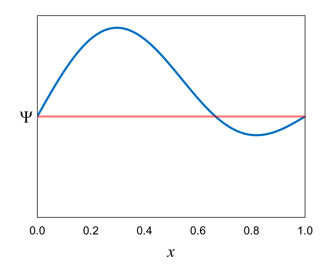
Figure 19 shows a wavefunction that is an equal superposition of the first two definite-energy eigenfunctions (ψ₆ and ψ₂₄). The probability amplitudes (c₆ and c₂₄) are both 1/√2.

Ψ = (1/√2)(ψ₆) + (1/√2)(ψ₂₄)

If we measure the energy of the electron in a box represented by this wavefunction, the probability of measuring each definite energy is the square of the probability amplitude = (1/√2)² = 1/2. When we measure the energy of the electron, the wavefunction collapses to the definite-energy eigenfunction corresponding to the measured definite energy.

Suppose we know that an electron in a box is represented by the wavefunction shown in Figure 19, but we do not already know the probability amplitudes for the definite-energy eigenfunctions making up the superposition. We want to know the probability amplitudes so that we will know the probabilities for measuring various definite-energy values. We can use the same technique we discussed for position and momentum. The probability amplitude for any definite-energy eigenfunction is equal to the inner product of the definite-energy eigenfunction and the wavefunction. For the wavefunction shown in Figure 19, the inner product of ψ₆ and Ψ, and the inner product of ψ₂₄ and Ψ, are both 1/√2.

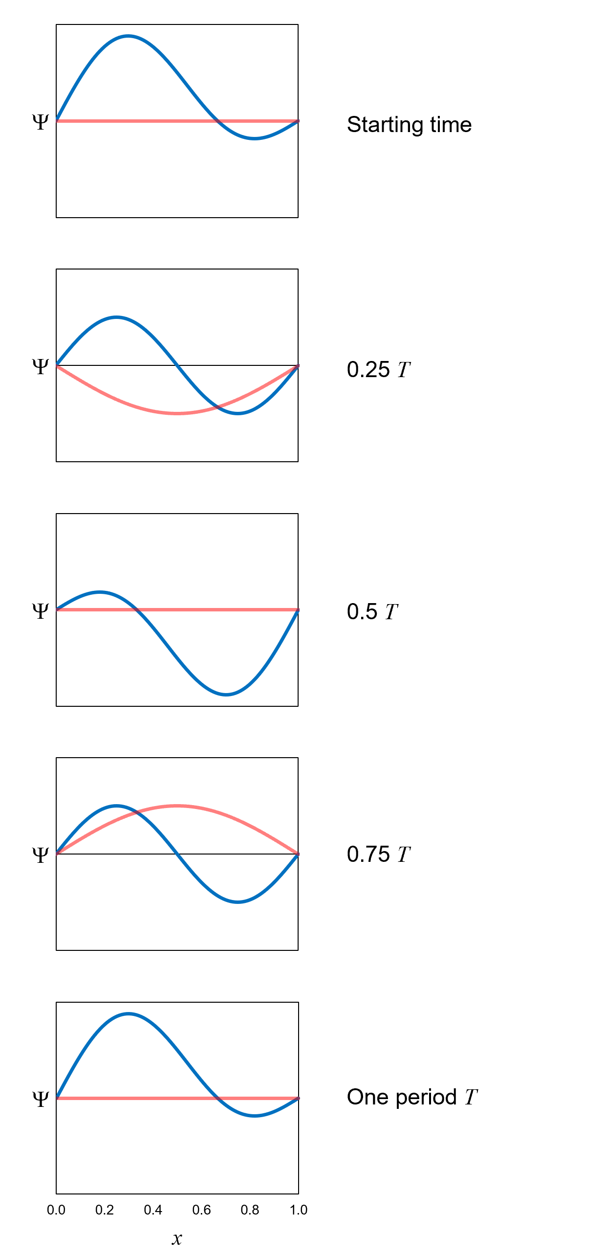
Figure 20 shows how the wavefunction that is an equal superposition of the first two definite-energy eigenfunctions oscillates over time according to the Schrödinger equation. The period of oscillation T is on the order of 1 × 10⁻¹⁶ seconds (pretty dang fast!).

Recap for an electron in a box with a focus on the energy of the electron:

• If the electron has a definite energy, then it is represented by a definite-energy eigenfunction ψ like the ones shown in Figure 18.
• Because the electron is confined, the possible values of definite energy are discrete and include a non-zero ground-state value. This is different from the possible values of definite position and definite momentum, which are both always continuous.
• Any electron wavefunction Ψ is a superposition of definite-energy eigenfunctions ψ. In the superposition, each definite-energy eigenfunction is multiplied by a probability amplitude.
• We can determine the value of a probability amplitude by calculating the inner product of the definite-energy eigenfunction ψ and the wavefunction Ψ.
• The probability of measuring a particular definite energy is the square of the probability amplitude corresponding to the particular definite-energy eigenfunction.
• Upon measurement of energy, the wavefunction Ψ collapses to one of the definite-energy eigenfunctions ψ that made up the superposition before measurement.