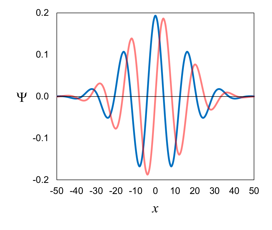
In this chapter we will learn what an electron wavefunction tells us about the position of the electron. We will use the electron wavefunction shown in Figure 3 at t₁, which is reproduced below in Figure 5. This is a wavefunction in position space; it is a function of x on the horizontal axis.

The units for position are Angstroms. One Angstrom = 1 × 10⁻¹⁰ meters, which is roughly the size of a hydrogen atom. On this website, all dimensions of length are expressed in Angstroms.

You do not need to know the units for the wavefunction to understand the material covered on this website. In case you are wondering, however, the units for a wavefunction in one-dimensional position space are 1/√Angstrom. You can look forward to these units making sense as you go on to learn more about quantum mechanics.

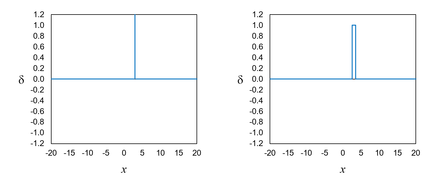
Before considering what the wavefunction tells us about the position of the electron, let’s take a step back and consider what the quantum state would look like if the electron had a definite position. Figure 6, left, shows a function representing an electron with a definite position. We call this function a position eigenfunction, δ. The value of the definite position is called the eigenvalue. We say that when an electron is in such a quantum state, it is in a definite-position eigenstate with a corresponding eigenfunction and eigenvalue. Think of an eigenstate as a package-deal: every eigenstate comes with an eigenfunction and an eigenvalue.

We will not use the term position eigenvalue much on this website. We will say definite-position value instead. The same will go for momentum and energy in later chapters.

The definite-position value in Figure 6, left, is x = 3. The height of δ₃—the eigenfunction corresponding to the definite position of 3—is off the chart at x = 3 and zero everywhere else. Theoretically, if an electron has an exact position, its eigenfunction is infinitely tall and infinitesimally narrow at the exact position.

It will be easier to understand what’s going on if we assume that the position variable is discrete rather than continuous. Instead of allowing x to have any value, we will limit it to discrete values like 2, 3, 4, etc. We can interpret this to mean that if an electron has a definite position of 3, then really the electron is somewhere between 2.5 and 3.5. Figure 6, right, shows a simple approximation of the eigenfunction. It is a tall, thin rectangle with a height of 1 and a width of 1 at x = 3. Its value is zero everywhere else.

Now I have a proposition for you: We can use definite-position eigenfunctions as scalable building blocks to construct the wavefunction shown in Figure 5.

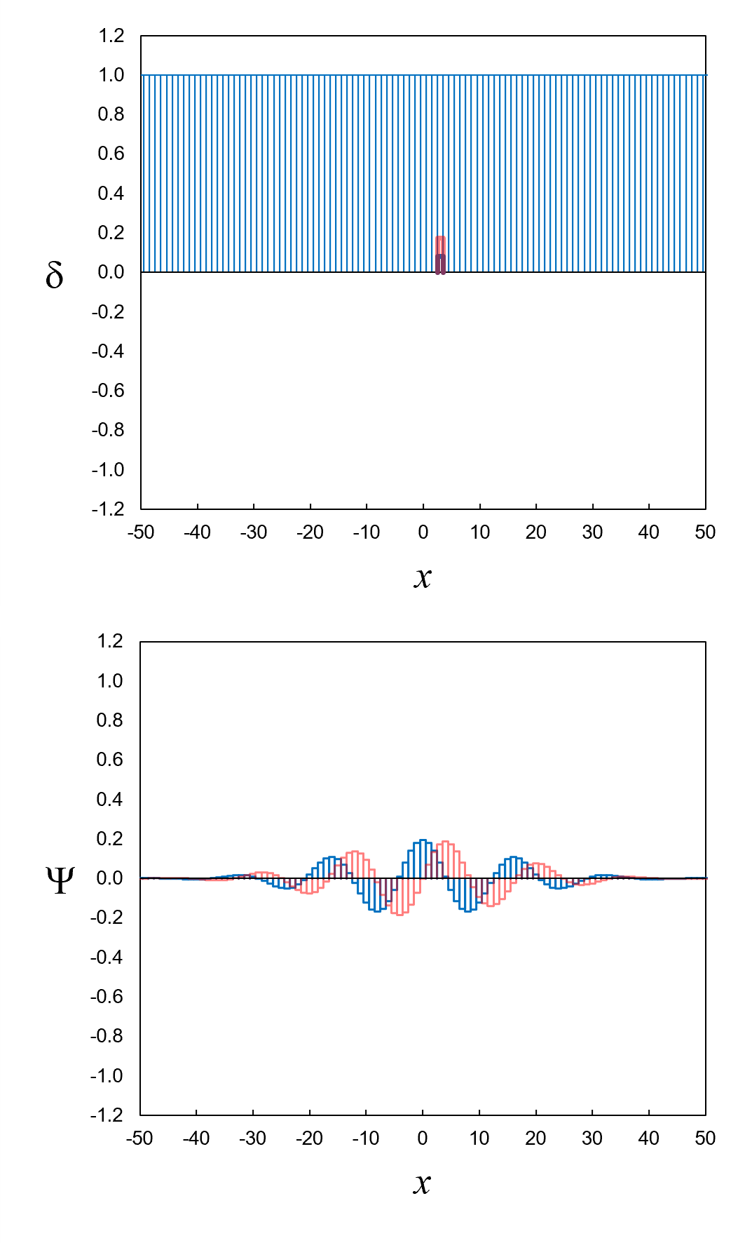
Figure 7, top, shows a set of neighboring definite-position eigenfunctions (light blue lines). There are 101 of them ranging from x = −50 to x = 50.

We can create the wavefunction in Figure 5 in two steps:

1. Multiply each definite-position eigenfunction δ by an amplitude a to get a new function aδ. The amplitudes are complex numbers.
2. Add up the functions resulting from step 1.

For step 1, assume for now that we already know the amplitudes needed to create the wavefunction. We have a list of 101 amplitudes (a₋₅₀ through a₅₀), one for each definite-position eigenfunction from δ₋₅₀ to δ₅₀.

In our list, the complex amplitude a₃ for the definite-position eigenfunction δ₃ is 0.080 + 0.173i. When we multiply δ₃ by a₃, we get a new function a₃δ₃ that is 0.080 + 0.173i at x = 3 (where δ₃ = 1) and zero everywhere else (where δ₃ = 0). Figure 7, top, shows the new function a₃δ₃ as a blue line (real part) plus a red line (imaginary part).

We do the same thing to make the new functions (a₋₅₀)(δ₋₅₀), (a₋₄₉)(δ₋₄₉), (a₋₄₈)(δ₋₄₈), etc.; again, assuming that we already know all of the amplitudes.

Step 2 is to add up the functions resulting from step 1. In equation form, this is

Ψ = (a₋₅₀)(δ₋₅₀) + (a₋₄₉)(δ₋₄₉) + (a₋₄₈)(δ₋₄₈) + ... + (a₅₀)(δ₅₀) = ∑a_xδ_x

Figure 7, bottom, shows the result of step 2 in graphical form. What we get is a very good approximation of the wavefunction in Figure 5.

The procedure we just used to construct the wavefunction in Figure 5 can be used to construct any electron wavefunction. This is a big deal. Show us an electron wavefunction of any shape, and we can build it by 1) scaling the definite-position eigenfunctions (i.e., multiplying them by complex numbers called amplitudes) and 2) adding up the resulting functions. There is a special name for this procedure: superposition. In quantum mechanics, we say that the electron wavefunction Ψ is a superposition of definite-position eigenfunctions δ.

All of this great, but we have not yet answered the question, where is the electron represented by the wavefunction? The answer is, the electron is not in any single position. It is in a superposition of the definite positions used to construct the wavefunction! If we were to measure the electron’s position, we could find it at any position x where the wavefunction is not zero.

This may feel like a hopeless situation, but it is not that bad. The amplitude that we use to scale a particular definite-position eigenfunction tells us something about the probability of finding the electron at that definite position upon measurement. Here is how it works: The probability of finding the electron at position x is the square of the amplitude a_x. The physicist Max Born figured this out in 1926. From here on we will call the amplitudes probability amplitudes.

For example, the probability amplitude a₃ corresponding to x = 3 is 0.080 + 0.173i. Using the equation in Figure 4 for squaring complex numbers, the square of a₃ is (0.080)² + (0.173)² = 0.036 = 3.6%. This is the probability of measuring the electron to be at the definite position of 3.

The overall probability of finding the electron somewhere within the bounds of the wavefunction has to be 1.0. We are certainly going to find it somewhere! This fact can be expressed as

|a₋₅₀|² + |a₋₄₉|² + |a₋₄₈|² + ... + |a₅₀|² = 1.0

Pause and let this sink in. In classical mechanics, the classical state tells us exactly where the electron is. There is no uncertainty. In quantum mechanics, the quantum state—when represented by a wavefunction that is not a definite-position eigenfunction—tells us the probability of finding the electron at any position upon measurement. There is inherent uncertainty. We cannot get rid of it. We have to give up on expecting to know precisely where the electron is before making a measurement.

We assumed above that we already knew the probability amplitudes needed to create the wavefunction in Figure 5. But what if we just have the wavefunction in Figure 5? How can we tell what the probability amplitudes are for the definite-position eigenfunctions involved in the superposition?

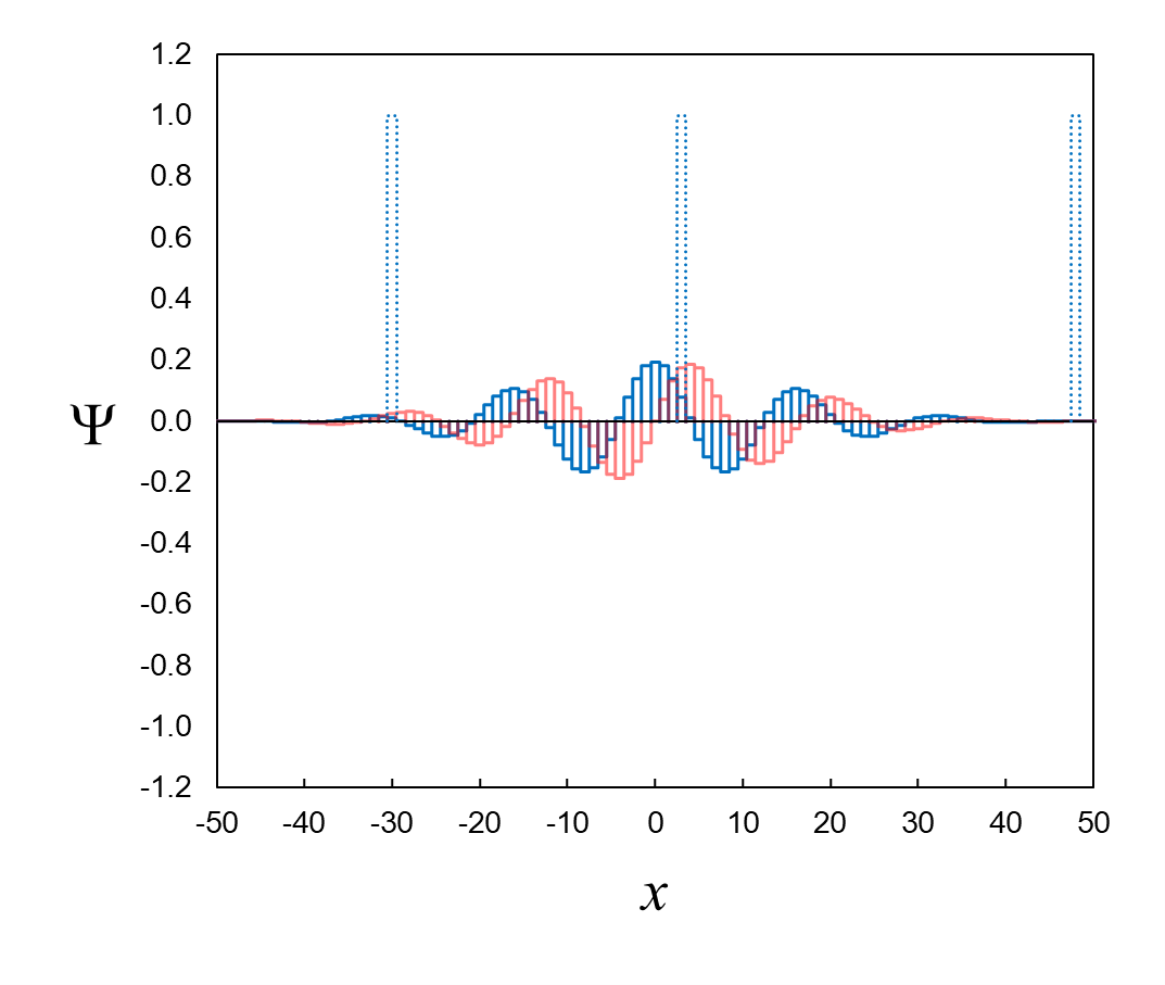
For any definite-position eigenfunction, the probability amplitude is equal to the overlap between the wavefunction and the definite-position eigenfunction. We can get a sense for the overlap visually. In Figure 8, the overlaps for the definite-position eigenfunctions δ₋₃₀, δ₃, and δ₄₈ appear to be relatively small, large, and insignificant, respectively.

There is a way to calculate the overlap. It is equal to the inner product of a definite-position eigenfunction δ and the wavefunction Ψ. The inner product calculation involves integral calculus. You basically multiply the wavefunction by the definite-position eigenfunction to get a new function, then evaluate the area under the new function. If we calculate the inner product of δ₃ and the Ψ in Figure 5, we get 0.080 + 0.173i. This is the probability amplitude a₃. Inner product = overlap = probability amplitude.

We have talked about the probabilities of finding the electron at definite positions upon measurement. What happens when we actually perform the measurement? Before the measurement, the electron is represented by a wavefunction Ψ that is a superposition of many definite-position eigenfunctions δ. Upon measurement, the wavefunction Ψ collapses to (i.e., becomes) one of the definite-position eigenfunctions δ. The state of the electron is now represented by the single definite-position eigenfunction corresponding to where we found the electron upon measurement.

Recap:

• If an electron has a definite position, then it is represented by a definite-position eigenfunction δ like the ones shown in Figure 6, left or right.
• Any electron wavefunction Ψ is a superposition of definite-position eigenfunctions δ. In the superposition, each definite-position eigenfunction is multiplied by a probability amplitude.
• We can determine the value of a probability amplitude by calculating the inner product of the definite-position eigenfunction δ and the wavefunction Ψ.
• The probability of measuring the electron to be at a particular position is the square of the probability amplitude corresponding to the particular definite-position eigenfunction.
• Upon measurement of position, the wavefunction Ψ collapses to one of the definite-position eigenfunctions δ that made up the superposition before measurement.