In the previous chapter we learned what an electron’s quantum state looks like when the electron has a definite position. We then learned that we can express any electron wavefunction as a superposition of definite-position eigenfunctions. In this chapter we are going to see that we can also express any electron wavefunction as a superposition of definite-momentum eigenfunctions.

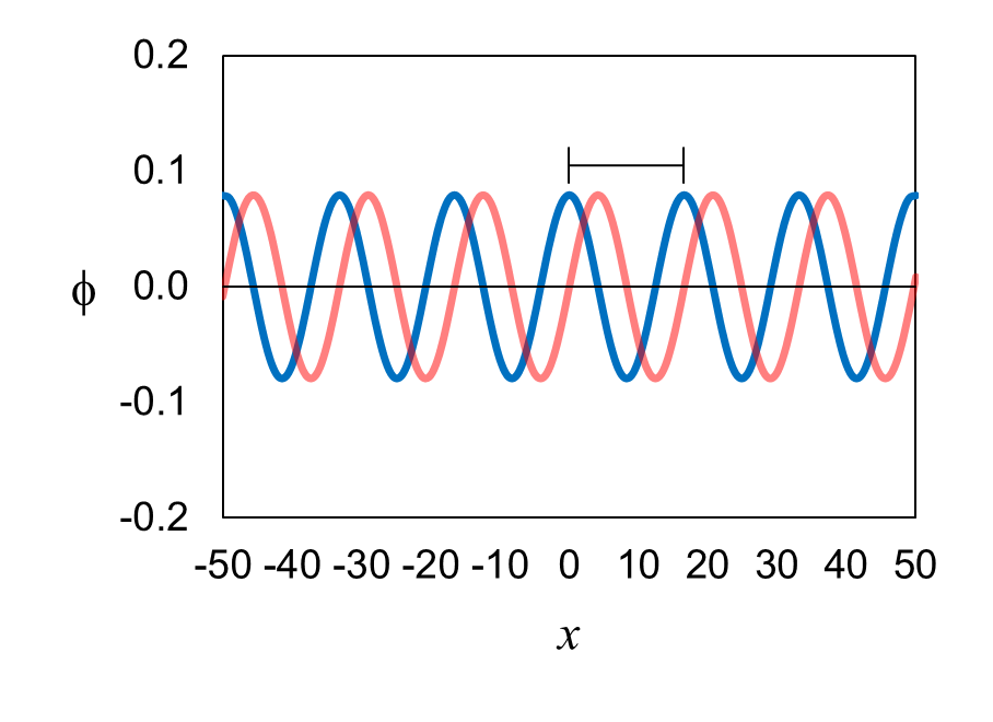
Figure 9 shows the eigenfunction ϕ for an electron with a definite momentum p. It is a wave with both a real part (blue) and an imaginary part (red). The wave extends to the left to x = −∞ and to the right to x = +∞.

If this is the first time you are seeing a definite-momentum eigenfunction, you are justified in wondering how in the world we get momentum from this. The answer dates back to 1923, when the physicist Louis de Broglie asked the question: If light can be thought of as both a particle (a photon) and a wave, why not think of any quantum entity—let’s say an electron—as both a particle and a wave? In the wave representation of an electron, the electron’s momentum p is related to the wavelength λ of the wave. The wavelength is the distance between neighboring peaks of the wave. De Broglie’s relationship is

p = h ∕ λ

In this relationship, h is Max Planck’s constant from 1900: h = 6.626 × 10^-34 Joule-seconds. A Joule is a unit of energy: 1 Joule = 1 kg⋅m²/s².

For the definite-momentum eigenfunction shown in Figure 9, the wavelength λ = 16.6 Angstroms = 1.66 × 10^-9 m, so the electron’s momentum p = 4.0 × 10^-25 kg⋅m/s. On this website, all values of momentum will be expressed as a multiplier of 10^-25 kg⋅m/s. For example, we will express 4.0 × 10^-25 kg⋅m/s as 4.0.

Let’s see how we can construct the electron wavefunction in Figure 5, Chapter 4 as a superposition of definite-momentum eigenfunctions.

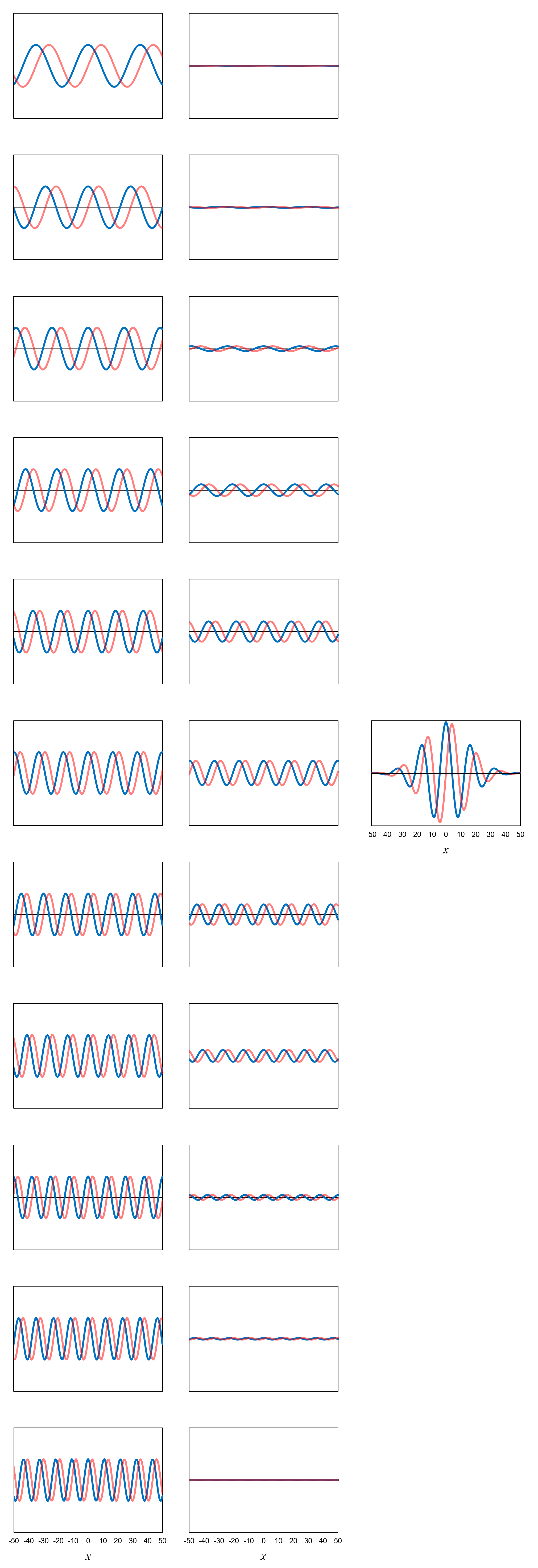
Figure 10, left column, shows a set of eleven definite-momentum eigenfunctions for momentum values ranging from 1.9 (top) to 6.1 (bottom). As we did for position, we are limiting momentum to discrete values (even though momentum is actually a continuous variable). The increment between the discrete values is 0.42 (which, by the way, has been built into the eigenfunctions shown). We can interpret this to mean that if an electron has a definite momentum of 4.0, then really its momentum is somewhere between 3.79 and 4.21.

Note that the wavelength of the definite-momentum eigenfunctions decreases as the momentum increases in accordance with de Broglie’s relationship.

We can create the wavefunction in Figure 5 using the same two steps we used in Chapter 4 when dealing with definite-position eigenfunctions:

1. Multiply each definite-momentum eigenfunction ϕ by a probability amplitude b to get a new function bϕ.
2. Add up the functions resulting from step 1.

For step 1, assume again that we already know the probability amplitudes needed to create the wavefunction in Figure 5. Figure 10, center column, shows the new functions that we get by multiplying the eleven definite-momentum eigenfunctions ϕ by their respective probability amplitudes b.

Step 2 is to add up the functions resulting from step 1. In equation form, this is

Ψ = (b_1.9)(ϕ_1.9) + (b_2.3)(ϕ_2.3) + (b_2.7)(ϕ_2.7) + ... + (b_6.1)(ϕ_6.1) = ∑b_pϕ_p

Figure 10, right, shows the result of step 2 in graphical form. We get again the wavefunction in Figure 5!

An amazing thing has happened here. The definite-momentum eigenfunctions all extend to plus and minus infinity in the x direction. After scaling them (i.e., multiplying them by probability amplitudes) then adding up the results, however, the resulting wavefunction goes to zero around x = ±50.

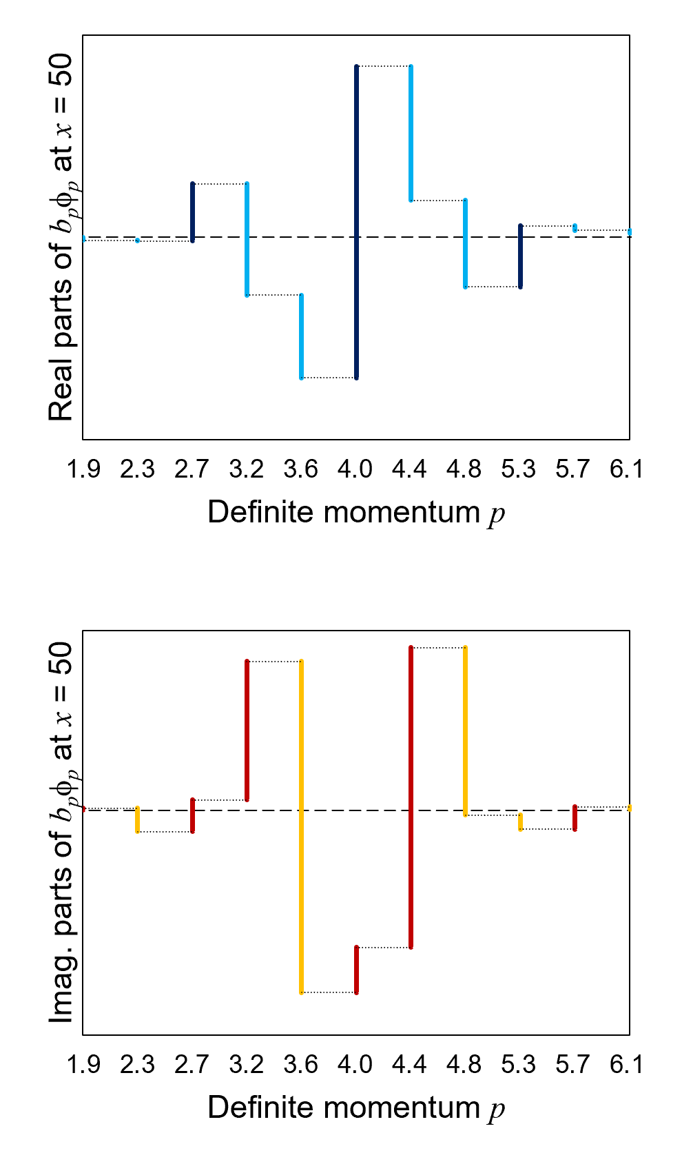
Figure 11 shows the summation of the real parts (top graph) and imaginary parts (bottom graph) of the eleven values of b_pϕ_p at x = 50. The summation accumulates from the left side at b_1.9ϕ_1.9 to the right side at ∑b_pϕ_p (all, again, at x = 50). For both the real and imaginary parts, the summation equals approximately zero (the horizontal dashed line) on the right side.

The phenomenon described above is called interference. The interference is destructive where the waves tend to cancel one another out (around x = ±50). The interference is constructive where the waves tend to amplify one another (around x = 0).

We can generalize here like we did when considering definite-position eigenfunctions. Show us any electron wavefunction, and we can build it by 1) scaling the definite-momentum eigenfunctions (i.e., multiplying them by probability amplitudes) and 2) adding up the resulting functions. We learned in Chapter 4 that any electron wavefunction Ψ is a superposition of definite-position eigenfunctions δ. It is also true that any electron wavefunction Ψ is a superposition of definite-momentum eigenfunctions ϕ.

Can you guess how we figure out the probability of finding the electron to have any one of the definite momenta upon measurement? We square the probability amplitudes. For example, the probability amplitude b_4.0 corresponding to p = 4.0 is 0.582 + 0i (the imaginary part is zero). The probability of measuring the electron to have this definite momentum is (0.582)² + (0)² = 0.339 = 33.9%.

We assumed above that we already knew the probability amplitudes for the definite-momentum eigenfunctions needed to create the electron wavefunction in Figure 5. We can determine the definite-momentum eigenfunction probability amplitudes for any electron wavefunction by using the same method we discussed for position. The probability amplitude for a definite-momentum eigenfunction is equal to the inner product of the definite-momentum eigenfunction ϕ and the wavefunction Ψ. The inner product is calculated the same way as described for position: basically, multiply the wavefunction by the definite-momentum eigenfunction to get a new function, then evaluate the area under the new function.

Measurement for momentum works the same way as measurement for position. Before measurement, the electron is represented by a wavefunction that is a superposition of many definite-momentum eigenfunctions. Upon measurement, the wavefunction collapses to one of the definite-momentum eigenfunctions. The state of the electron is now represented by the single definite-momentum eigenfunction corresponding to the measured momentum of the electron.

The recap is basically the same as that for position. The only difference is that we are talking about momentum instead of position.

• If an electron has a definite momentum, then it is represented by a definite-momentum eigenfunction ϕ like the one shown in Figure 9.
• Any electron wavefunction Ψ is a superposition of definite-momentum eigenfunctions ϕ. In the superposition, each definite-momentum eigenfunction is multiplied by a probability amplitude.
• We can determine the value of a probability amplitude by calculating the inner product of the definite-momentum eigenfunction ϕ and the wavefunction Ψ.
• The probability of measuring a particular momentum is the square of the probability amplitude corresponding to the particular definite-momentum eigenfunction.
• Upon measurement of momentum, the wavefunction Ψ collapses to one of the definite-momentum eigenfunctions ϕ that made up the superposition before measurement.

Before moving on, let’s talk about the energy E of the electron we have been considering: one moving along with no force acting on it. As described above, when we measure the electron’s momentum, the wavefunction collapses to a definite-momentum eigenfunction with its corresponding definite-momentum value. For an electron moving along with no force acting on it, there is a one-to-one relationship between momentum and energy. If the measured definite momentum is p, then the definite energy is p²/2m (which is the classical expression for kinetic energy). This will not be the case when an electron is confined by forces, as we will see in Chapters 9 and 10.