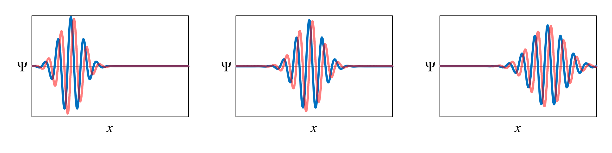
Figure 3 in Chapter 2 shows how the wavefunction for an electron moving from left to right with no force acting on it changes with time. The time-evolution of the wavefunction is reproduced in Figure 13. Notice that the shape of the wavefunction changes over time: it spreads out. This behavior is accurately predicted by the Schrödinger equation, which was developed by the physicist Erwin Schrödinger in 1926. The Schrödinger equation is the dynamical law governing how wavefunctions change over time.

Before talking about the Schrödinger equation, let’s discuss a dynamical law we use in classical mechanics: Newton’s second law. You may be familiar with the version F = ma. Force equals mass times acceleration. There is another way to express Newton’s second law: dp/dt = F. The change in an object’s momentum (dp) with respect to time (dt) is equal to the force acting on it. This dynamical law tells us how an object’s momentum changes with time.

The dynamical law we use in quantum mechanics is the Schrödinger equation, which is shown in Figure 14.

On the left side of the equation is ∂Ψ/∂t, which is the change in the wavefunction with respect to time. This is what we want to know: how does the wavefunction change over time.

Note that wavefunctions in position space are functions of position and time. If we were being explicit, we would write Ψ(x,t) instead of just Ψ. It would be easier to see, then, that ∂Ψ(x,t)/∂t—the change in the wavefunction with respect to time—can be evaluated at different values of x. A wavefunction can change with time differently at different values of x.

The right side of the equation has two terms, one related to kinetic energy and one related to potential energy. Kinetic energy and potential energy are the two components of total energy. Assume that for a particular problem, we know the things on the right side of the equation at a particular time. We know the wavefunction Ψ at the particular time (as a function of x), the mass m of the quantum entity, and the potential energy V at the particular time (as a function of x).

Of the two terms on the right side of the equation, let’s start with the potential energy term. For the case of our electron moving from left to right with no force acting on it, the potential energy is constant everywhere (so, without loss of generality, we can assume it is zero). In Chapter 8, we will see how a potential energy gradient is related to force. In Chapters 9 and 10, we will see the effect of varying (i.e., not-constant) potential energy distributions when we discuss an electron in a box and an electron in a hydrogen atom.

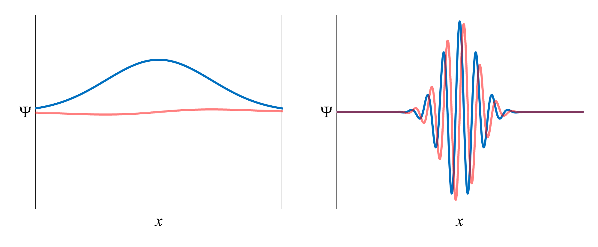
The kinetic energy term in the Schrödinger equation depends on the curvature of the wavefunction. The curvature is how much the slope of the wavefunction changes over x. Figure 15 shows two example wavefunctions.

• The one on the left has relatively low curvature. Its slope changes gradually with x. This wavefunction has relatively low kinetic energy.
• The one on the right has relatively high curvature. Its slope changes rapidly with x. This wavefunction has relatively high kinetic energy.

What, then, does the Schrödinger equation tell us? It tells us that the rate of change of a wavefunction with respect to time depends on the total energy of the wavefuncion. The higher the total energy, the faster the time-evolution of the wavefunction.

Here is how we can evolve a wavefunction Ψ over time. Once we know both Ψ and ∂Ψ/∂t (from the Schrödinger equation) at one time (t₀), we can determine (approximately) what Ψ will be a short time later (at t₁):

Ψ(t₁) ≈ Ψ(t₀) + [∂Ψ(t₀) ∕ ∂t] Δt

where
Δt = t₁ − t₀
The approximation gets better as Δt gets shorter.

In the paragraph above, "determine" is a key word. Wavefunctions evolve deterministically via the Schrödinger equation when measurement is not involved. If we know Ψ at one time, then we can determine what it will be at any other time (assuming that we also know V over time). We only get inherently probabilistic outcomes upon measurement.